
Step by Step Instruction
- Drone + photogrammetry
- Point cloud transformation (Agisoft Metashape)
- Segment + clustering sediments (G3Point) < this is MATLAB code btw:(
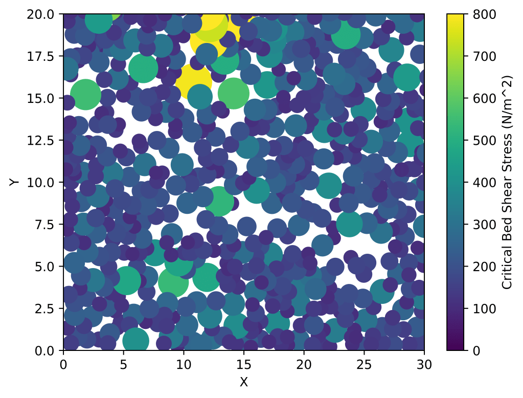
- XY + Z (Diameter) map with Python (I had to convert MATLAB to Python, instruction on how below)
Instruction on transforming G3Point to Python cluster scatterplot (doing this, bc I’m probably going to forget how to do it in like a week).
%% Install G3Point, install required toolboxes (provided in Github), make sure the code runs, and make a MATLAB file with the code below in the G3Point directory. It should output a text file called rawdata.txt

clearvars;
addpath('Utils','-end');addpath('Utils/quadfit','-end');  addpath('Utils/geom3d/geom3d/','-end');

%% Inputs
param.ptCloudname='';% 'Mangaweka.ply' 'Otira_1cm_grains.ply' 'Test1_clean_registered.ply'
if isempty(param.ptCloudname)==1;[param.ptCloudname,param.ptCloudpathname] = uigetfile('*.ply','Select the *.ply point cloud file');end

%% Loading data
[ptCloud,param]=loadptCloud(param);

%% Algorithm parameters - Compute point cloud size and scaling of the algorithm
% Load parameters
param=defineparameters(ptCloud,param);
% Display algorithm header
displayheader(ptCloud,param);

%% Denoise and decimate point cloud
% Denoise
if param.denoise==1;  ptCloud = pcdenoise(ptCloud); end
% Decimate
if param.decimate==1; ptCloud = pcdownsample(ptCloud, 'gridAverage', param.res);end

%% Remove the point that are localized in local minima (multiscale) to ease segmentation and delimitation of grains
if param.minima==1
    % Compute distance to local plan using a multiscale approach
    [dist]=disttoplanemultiscale(ptCloud,param.minscale,param.maxscale,param.nscale);
    % Identify and remove local minimas
    ind=find(dist<prctile(dist,95));
    x=ptCloud.Location(:,1); y=ptCloud.Location(:,2); z=ptCloud.Location(:,3); ptCloud = pointCloud([x(ind) y(ind) z(ind)]);
end


%% Rotate and detrend the point cloud
if param.rotdetrend==1
    % Detrending assume that the plan is already orientated with the grains
    % upward in the z-direction (but the point cloud can be tilted compared to
    % the horizontal plan)
    [A,B,C,distsigned,distabs]=fitplan(ptCloud.Location);Normal=[-A -B 1]; [Normal]=adjustnormals3d(0,0,0,Normal,[0 0 1e32]); R=vec2rot(Normal, [0 0 1], 'Rik'); meanptCloud=mean(ptCloud.Location); xyzPoints=(R*(ptCloud.Location-meanptCloud)')'+meanptCloud; ptCloudRot = pointCloud(xyzPoints);
    % Then, if needed, remove a polynomial trend from the ptCloud
    x=ptCloudRot.Location(:,1);y=ptCloudRot.Location(:,2);z=ptCloudRot.Location(:,3); A = [ones(size(x)) x y x.^2 x.*y y.^2] \ z; z= z -( A(1) + A(2).*x + A(3).*y + A(4).*x.^2 + A(5).*x.*y + A(6).*y.^2); ptCloudRot = pointCloud([x y z]);
end


%% Show the clean point cloud
    % Plot
    if param.iplot==1;pcshow(ptCloudRot.Location,ptCloudRot.Location(:,3));set(gcf,'color','w');set(gca,'color','w');axis equal tight;cb = colorbar('north');set(cb,'position',[.5 .75 .1 .02]);ylabel(cb,'Elevation');axis off;end
    if param.saveplot==1 && param.iplot==1;nom=[param.figurefolder 'elevation'];print('-djpeg','-r1500',nom);savefig(nom);close;end; %print('-dpdf','-painters',nom);

%% Segment and cluster the point cloud into a point cloud of potential grains
% Find neighbors of point cloud
[indNeighbors,D]=knnsearch(ptCloud.Location,ptCloud.Location,'K',param.nnptCloud+1);indNeighbors=indNeighbors(:,2:end);D=D(:,2:end);
% determine node surface
surface=pi.*min(D,[],2).^2;
% Compute normals and force them to point towards positive Z
normals = pcnormals(ptCloud,param.nnptCloud);[normals]=adjustnormals3d(ptCloud.Location(:, 1),ptCloud.Location(:, 2),ptCloud.Location(:, 3),normals,[mean(ptCloud.Location(:,1)), mean(ptCloud.Location(:,2)),10000]);
% Initial segmentation with Fastscape
[labels,nlabels,labelsnpoint,stack,nstack,ndon,isink]=segment_labels(ptCloudRot,param,indNeighbors);cmaplabels=rand(nlabels,3);
    % Plot
    if param.iplot==1;pcshow(ptCloud.Location,labels);colormap(cmaplabels);hold on;set(gcf,'color','w');set(gca,'color','w');axis equal tight;hold on;plot3(ptCloud.Location(isink,1),ptCloud.Location(isink,2),ptCloud.Location(isink,3),'.r');axis off;end
    if param.saveplot==1 && param.iplot==1;nom=[param.figurefolder 'labels_ini'];print('-djpeg','-r500',nom);savefig(nom);close;end; %print('-dpdf','-painters',nom);
% Cluster Labels to prevent over-segmentation
[labels,nlabels,stack,isink]=cluster_labels(ptCloud,param,indNeighbors,labels,nlabels,stack,ndon,isink,surface,normals);cmaplabels=rand(nlabels,3);
    % Plot
    if param.iplot==1;pcshow(ptCloud.Location,labels);colormap(cmaplabels);hold on;set(gcf,'color','w');set(gca,'color','w');axis equal tight;hold on;plot3(ptCloud.Location(isink,1),ptCloud.Location(isink,2),ptCloud.Location(isink,3),'.r');axis off;end
    if param.saveplot==1 && param.iplot==1;nom=[param.figurefolder 'labels_cluster'];print('-djpeg','-r500',nom);savefig(nom);close;end; %print('-dpdf','-painters',nom);

%% Clean the segmentation
if param.clean==1
    % Clean the segmentation
    [labels,nlabels,stack,isink]=clean_labels(ptCloud,param,indNeighbors,labels,nlabels,stack,ndon,isink,surface,normals);
    % Plot
    if param.iplot==1;pcshow(ptCloud.Location,labels);colormap(cmaplabels);hold on;set(gcf,'color','w');set(gca,'color','w');axis equal tight;hold on;plot3(ptCloud.Location(isink,1),ptCloud.Location(isink,2),ptCloud.Location(isink,3),'.r');axis off;end
    if param.saveplot==1 && param.iplot==1;nom=[param.figurefolder 'labels_clean'];print('-djpeg','-r500',nom);savefig(nom);close;end; %print('-dpdf','-painters',nom);
end

%% Generate a Pebble structure
for i=1:nlabels;ind=find(labels==i);Pebble(i).Location=ptCloud.Location(ind,:);Pebble(i).ind=ind;Pebble(i).surface=surface(ind);end

%% Fitting cuboids (no dip allowed but azimuth is optimized)
% Fit
display(['--- FITTING CUBOIDS TO GRAINS']);
tic;for k=1:nlabels;Cuboidm(k)=pcfitcuboid(pointCloud(Pebble(k).Location));end;toc
    % Plot
    if param.iplot==1
    h=figure;plot3(ptCloud.Location(:,1),ptCloud.Location(:,2),ptCloud.Location(:,3),'.k','MarkerSize',1);axis equal tight;hold on;axis off
    for j=1:nlabels;  plot(Cuboidm(j));  end; cb = colorbar('north');set(cb,'position',[.5 .75 .1 .02]);ylabel(cb,'Labels');end; % How to plot colored cuboids?
    if param.saveplot==1 && param.iplot==1;nom=[param.figurefolder 'fitted_cuboids'];print('-djpeg','-r500',nom);savefig(nom);close;end

%% Fitting ellipsoids
% fit
[Ellipsoidm]=fitellipsoidtograins(Pebble,param,nlabels);
    % Plot
    if param.iplot==1
    h=figure;plot3(ptCloud.Location(:,1),ptCloud.Location(:,2),ptCloud.Location(:,3),'.k','MarkerSize',1);axis equal tight;hold on;axis off
    for j=1:nlabels;  try if Ellipsoidm(j).fitok==1; plot_ellipsoid_im(Ellipsoidm(j).p,'EdgeColor',cmaplabels(j,:)); end; end; end;cb = colorbar('north');set(cb,'position',[.5 .75 .1 .02]);ylabel(cb,'Labels');end;
    if param.saveplot==1 && param.iplot==1;nom=[param.figurefolder 'fitted_ellipsoids'];print('-djpeg','-r500',nom);savefig(nom);close;end


fid = fopen('rawdata.txt', 'w');
for j = 1:nlabels
    if Ellipsoidm(j).fitok == 1
        ellipsoid_fitok = Ellipsoidm(j).fitok;
        ellipsoid_Aqualityok = Ellipsoidm(j).Aqualityok;
        ellipsoid_p = Ellipsoidm(j).p;
        ellipsoid_c = Ellipsoidm(j).c;
        ellipsoid_r = Ellipsoidm(j).r;
        ellipsoid_q = Ellipsoidm(j).q;
        ellipsoid_R = Ellipsoidm(j).R;
        ellipsoid_axis1 = Ellipsoidm(j).axis1;
        ellipsoid_axis2 = Ellipsoidm(j).axis2;
        ellipsoid_axis3 = Ellipsoidm(j).axis3;
        ellipsoid_d = Ellipsoidm(j).d;
        ellipsoid_r2 = Ellipsoidm(j).r2;
        ellipsoid_V = Ellipsoidm(j).V;
        ellipsoid_A = Ellipsoidm(j).A;

        % Write ellipsoid parameters to the file
        fprintf(fid, 'p: %f\n', ellipsoid_p);
        fprintf(fid, 'c: %f\n', ellipsoid_c);
        fprintf(fid, 'r: %f\n', ellipsoid_r);
        fprintf(fid, 'q: %f\n', ellipsoid_q)d
        fprintf(fid, 'r2: %f\n', ellipsoid_r2);
        fprintf(fid, 'V: %f\n', ellipsoid_V);
        fprintf(fid, 'A: %f\n', ellipsoid_A);
        fprintf(fid, '\n');
    end
end
fclose(fid);

%csvwrite('x_location.csv', ptCloud.Location(:,1));
%csvwrite('y_location.csv', ptCloud.Location(:,2));
Import the rawdata.txt file to python and run it using the code below.
import matplotlib.pyplot as plt
os.chdir('/Users/braydennoh/anaconda3/G3Point/G3point')

sediment_data = []
current_sediment = {}

with open('rawdata.txt', 'r') as file:
    for line in file:
        line = line.strip()  # Remove leading/trailing whitespaces
        if line.startswith('p:'):
            current_sediment['p'] = float(line.split(':')[1].strip())
        elif line.startswith('c:'):
            if 'c' not in current_sediment:
                current_sediment['c'] = []
            current_sediment['c'].append(float(line.split(':')[1].strip()))
        elif line.startswith('r:'):
            current_sediment['r'] = float(line.split(':')[1].strip())
        elif line.startswith('q:'):
            current_sediment['q'] = float(line.split(':')[1].strip())
        elif line.startswith('r2:'):
            current_sediment['r2'] = float(line.split(':')[1].strip())
        elif line.startswith('V:'):
            current_sediment['V'] = float(line.split(':')[1].strip())
        elif line.startswith('A:'):
            current_sediment['A'] = float(line.split(':')[1].strip())
        elif line == '':
            if current_sediment:
                sediment_data.append(current_sediment)
                current_sediment = {}

# Extract x, y, and average r values for the XY map
x_values = []
y_values = []
r_values = []

for sediment in sediment_data:
    x_values.append(sediment['c'][0])
    y_values.append(sediment['c'][1])
    r_values.append(sediment['r'])

# Set the size of the markers based on the sediment diameter
marker_sizes = [r * 500 for r in r_values]

# Create the XY map with increased marker size
plt.scatter(x_values, y_values, c=r_values, vmin=0, vmax=2,cmap='turbo', s=marker_sizes)
plt.colorbar(label='Sediment Diameter (m)')
plt.xlabel('X')
plt.ylabel('Y')
plt.xlim([0, 30])
plt.ylim([0, 20])
plt.show()